
Theory of Credit Risk Model
Risk
Consequences of Uncertainty
Dimensions of Risk
- Event: what has to happen for the Risk to occur
- Duration: for how long are we exposed to this Risk
- Frequency: Probability or Rate of the Risk event occuring
- Severity: Magnitude of the consequences
- Correlation: Relationship with other Risk Events
- Capital: Reseves needed to support Risk
Uncertainty to each dimension
- Event: The cause could be uncertain
- Duration: The exposure could be uncertain
- Frequency: The true prob / rate could be uncertain
- Severity: The size of consequence could be uncertain
- Correlation: Relationships could be uncertain and subject to change
- Capital: Reserves might only give a level of confidence and not certainty
For Example) Life Insurance
- Exclusions to control for event uncertainty
- Term Assurance to control for duration uncertainty
- Actuarial Modeling to try reduce rate uncertainty
- Fixed Benefits to control severity uncertainty
- Sell Life Annuities to get diversification and offsetting benefits
- Pool multiple similar risks to increase capital confidence(Flip coin)
STANDARD APPROACH
-
Observe a population of size n for duration T
-
Count number of risk events that occur over duration T
\[Frequency = \frac{\#\ of\ risk\ events}{n}\] -
Observe size of loss from each risk event over duration T
\[Severity = \frac{\sum\\of\ all\ losses}{\#\ of\ risk\ events}\] \[Risk\ Price=Severity\times Frequncy\]
WHY MEASURE RISK
-
Measuring Risk helps us to Manage it efficiently
- low frequency & low severity: Retain
- low frequency & high severity: Transfer
- high frequency & low severity: Control
- high frequency & high severity: Avoid
- Do I want to take this Risk?
- How much should I pay to transfer it? What is a fair premium?
- What should my internal control budget be?
- How much capital do I need to retain this Risk?
Mathematical Properties of Risk Measures
-
Coherent: logical and consistenct
-
Coherent Axioms
-
Monotonicity: $if\ x_1 \lt x_2,\ then\ f(x_1) \lt f(x_2)$
-
Subadditivity: $f(x_1+x_2) \le f(x_1)+f(x_2)$
-
Positive Homogeneity: $f(kx)=kf(x)\ (k\ is\ a\ positive\ constant)$
-
Translation Invariance: $f(k+x)=k+f(x)\ (k\ is\ a\ constant)$
-
-
Convex:
\(f(tx_1 + (1-t)x_2) \le tf(x_1)+(1-t)f(x_2)\ (0\le t \le 1)\)
- What does this mean?
- Merge of Risks decreases Risk Profile
- Diversification
- Business units must stay within limits
- But what about Concentration & Systemic Risk
Credit Risk
- Event: 3rd Party fails to meet their obligation
- Duration: Specified by contract / type of instrument
- Frequency: Very low, normally only happens once(default)
- Severity: Very high, due to recovery, amount is uncertain
- Correlation: Low in stable times, High in distressed times(Economic conditions)
- Capital: None is isolation, but if using others’ money then reserves need to be established. Basel Accords
Identifying Credit Risk
- Lending Money to someone who then cannot repay
- Secured: Collateral
- Unsecured: No Collateral
- Buying Public Debt in form of Corporate or Government Bond
- Credit Spread Deteriorate(increases) -> price decreases
- Credit Spread Improve(decreases) -> price increases
- Counterparty Risk
- Insurance
- Derivatives
- Banking(Financial Institution) -> often not considered because protected by bailout
- Outsourcing Functions
Overview of Models
- Lending
- Face to Face Model(qualitative)
- Credit Score Model(quantitative)
- Due-Diligence Model
- Public Debt
- Merton Model
- KMV Model
- Two-State Model
- Jarrow-Lando-Turnbull Model
- Other Models
- Interest Rate Models: Frequency
- Value at Risk: Capital & Severity
- Copula’s: Correlation
Credit Modelling Challenges
- Lack of Data
- Bank don’t share their experience
-
Since Frequency is Low, Severity Data will be lacking even more(Hard to fit a distribution)
- Bond Durations
- Not all corporates have traded debt
- Those that do have differenct durations
- Different Model for 10yrs and 20yrs
- Credit Enhancements
- Guarantees by another party -> FRAUD
- Derivatives CDS, CDO -> ABUSE
- Changing Correlation
- Low when Stable Economy
- High during Recession
- Model mixing
- Differenct technique for Frequency & Severity
- Complexity joining and model risk
- Credit Rating Agency
- Conflicting information
- Business could game the system
- Conflict of Interest Risks
Face to Face Model
- Personal Meeting iwth Bank Manager
-
Questions & Requirements
- Security: Collateral or Surety
- Borrower: Degree, Job, Age, Record(Credit History, Criminal)
- Purpose: How will loan be used
- Financial Ratio: Cashflows, Assets, Liabilities
- Ecomony: Business Confidence, GDP, interests rates
- Decision to Approve / Reject
- Terms & Conditions
- Duration
- Interest Rate
- Risk to assess
- Default
- Recover
- Change
- Private Debt / Individual / Small Business
- Big Business: Team with more Questions & Requirements
Credit Score Model
- Automated Version of Face to Face model
- Act as a filter to save time
- Make decision to process loans fast
- Requires Data & Expertise to set Rules
-
Has blind spots, can’t consider everything
- Weighting to each factor is subjective
Introduction to Derivatives
- Derive their value from another underlying asset
- Purpose is to manage Market Risk
- Hedger: use to decrease Market Risk
- Speculator: use to increase Market Risk(Bet)
-
Hedgers Example
- Farmer wants to lock in price of sale
- Restaurant want to lock in price of costs
-
Speculators Example
- Asset manager A thinks oil price will go up
- Asset manager B thinks oil price will go down
-
Over the Counter
- Between two parties
- Customisable
- Counter Party Risk
- Difficult to close out early
-
Exchange Trade
- Both Parties go through a Clearing House
- Standardised
- Secure
- Easy to close out early
-
Types
- Futures, Forwards, Options, Swaps, Combinations, Exotics
-
Assumptions
-
Complete Market
- Everything has a price
- Transaction costs are zero
- Everyone has access to perfect information
-
No Arbitrage
- All assets are priced correctly
- Impossible to make a Risk Free Profit
-
Futures & Forwards Contracts
-
Future Delivery Price (K)
-
Future Delivery Date (T)
-
Value of Future at Delivery Date ($F_T$)
-
Long: $S_T-K$ (The buyer)
-
Short: $K-S_T$ (The seller)
-
Sub-Martingale
- \[F_T=S_T-K \ and \ E[S_T]=S_0e^{rT}\ (r\ is\ risk\ free\ rate)\]
-
$E[F_T]=0 \ (since\ F_0=0)$
-
$K=S_0e^{rT}$
- Expected future price is current price adjusted for T.V.M(Time Value of Money)
- If $K>S_0e^{rT}$ Long Asset and Short Future
- If $K < S_0e^{rT}$ Short Asset and Long Future
Call and Put Options
-
Long Call
- right, not obligation, to Buy asset at a specific Price at a specific Date
- Long Put
- right, not obligation, to Sell asset at a specific Price at a specific Date
- For both a Premium needs to be paid to the Short Party
- Short Option: Receive Premium and Obligation
- Long Option: Pay Premium and receive a Right
- Limit Downside Risk
- Maintain Upside Risk
Black Scholes Formula
- $C_0 = S_0N(d_1)-Ke^{-rT}N(d_2)$
-
$P_0=Ke^{-rT}N(-d_2)-S_0N(-d_1)$
-
$d_1= \frac{ln(S_0/K)+(r+\frac{\sigma^{2}}{2})T}{\sigma \sqrt{T}}$
- $d_2= \frac{ln(S_0/K)+(r-\frac{\sigma^{2}}{2})T}{\sigma \sqrt{T}}= d_1-\sigma\sqrt{T}$
Factors affecting Option Prices
-
Share Price: $as \ S_0\uparrow,\ C\uparrow\ P\downarrow$
-
Strike Price: $as \ K\uparrow,\ C\downarrow\ P\uparrow$
-
Time to expiry: $as \ T\uparrow,\ C\uparrow\ P\downarrow$
- Shares have a positive trend and this favors the call but hurts the put
- Volatility of share: $as \ \sigma\uparrow,\ C\uparrow\ P\uparrow$
- Options have limited downside but unlimited upside
- More risk makes both of them more valuable
- Risk free rate: $as \ r\uparrow,\ C\uparrow\ P\downarrow$
- Higher rate makes share grow faster
- Favors the call but hurts the put
Merton Model
History
- Robert Cox Merton
- Black Scholes Model
- Nobel Prize
- LTCM
- Robert Jarrow Student
- KMV extend Model
- Moody -> LossCalc / RiskCalc
IDEA
- Company is financed by Equity & Debt
- Equity: Vote & Unlimited Potential Return
- Debt: Fixed Return & Greater Security
- Assumption: No Dividends & Zero Coupon Bond
Formula
- $Value(0) = Equity(0) + Debt(0)$
- $Debt(T)=Min(Debt(0)*(1+i)^T,Value(T))$
- $Equity(T)=Max(Value(T)-Debt(T),0)$
- Equity is limited
-
If a company does badly -> $Debt(T)=Value(T), \ Equity(T)=0$
- Equity is like a Long Call on a company
- Debt is like a Short Put on a company
Related to Black Scholes Model
- $Equity(0)=C\ (Premium\ for\ a\ Call\ Option)$
-
$Debt(T)=K\ (Strike\ Price)$
- $i*Debt(0)=P\ (Premium\ for\ a\ Put\ Option)$
- $Value(T)=S_T\ (Share\ Price\ at\ Time\ T)$
- $Value(0)=S_0\ (Share\ Price\ at\ Time\ 0)$
Note Value(t) is Company’s Assets, Not Share Price
Just in Merton Model, Assets take place of Share Price in BS model
Also be aware, difficult to know Asset value of all times
We assume, we know volatility of the Asset value
- $Equity(0)=Value(0)N(d_1)-Debt(T)e^{-rT}N(d2)$
- $i*Debt(0)=Debt(T)e^{-rT}N(-d_2)-Value(0)N(-d_1)$
- $P(S_T<K)=N(-d_2)$
-
Thus Probability of Default at Time T is $P(Value(T) \le Debt(T)) = N(-d_2)$
- $Debt(0)=Debt(T)e^{-rT}-[Debt(T)e^{-rT}N(-d_2)- Value(0)N(-d_1)]$
- $Debt(0)=Debt(T)e^{-bT}\ (where\ b\ is\ implied\ interest\ rate)$
-
$Credit\ Spread\ is\ b-r$
- Merton Model tells us
- Probability of Default
- The Company’s Debt of various times
- The Credit Spread
Drawbacks of Merton Model
- Assuming Frictionless Market
- Deterministic Risk free rate
- Value of the company assets follow log Normal distribution with fixed growth & volatility
- Value is an obervable traded security
- Debt is a Zero Coupon Bond
- Debt has only one Default Opportunity
- Default only results in Liquidation
KMV Model
- Extends the Merton model idea
-
Probability of Default = $P(Value(T)<Debt(T))$
- Introduces the Distance to Default(DD)
- Number of standard of deviation that the company’s assets have to fall in value before they breach the Debt(T) threshold
-
$DD_0=\frac{Value(0)-Debt}{\sigma_{Value} \ Value(0)}$
- Use empirical data on company defaults and how these defaults link with the DD
- Can estimate PD over the coming year
- Normally we can’t observe Value nor $\sigma_{Value}$
- However
Ito's Lemmasays that
- Solve 2 simultaneous equations to get 2 numbers(above equation & bsm)
KMV Model vs Merton Model
- KMV allows for Coupon Paying Debt -> allows for more complex Liability Structures
- Value isn’t assumed to be observable, derived from price of shares
- Both are Structural Models, depend on share price. Thus market sentiment can have significant impact on results
Jarrow - Turnbull Model
History
- Robert Jarrow was a student of Robert Merton
- Merton used option pricing theory
-
Jarrow used markov process
- Both aim to calculate probability of default
- Credit Rating Agencies used Merton Model(KMV version)
- Jarrow uses credit ratings
- Jarrow is a sort of extension to Merton
IDEA
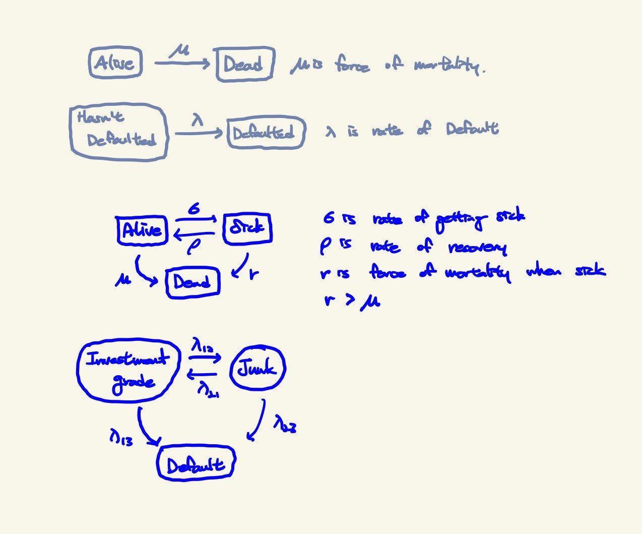
- Each Non-default state can move to every other state
- To estimate rates, use historical data
Results
- Time until default, allowing ofr credit deterioration
- Probability of losing Investment Grade status
Credit Migration Model Drawbacks
- Jarrow-Turnbull Model is an example
- See how Credit Ratings change over time
- Doesn’t explicitly need share information
-
Time-homogeneity is not realistic
- Studies show that a recently downgraded bond is more likely to downgrade in the future than one with same rating that has been there for longer
- Agencies don’t want to shock the market. There is also their outlook that some models dont’t consider
- Granularity vs Lack of data
- More states like Triple A- negative outlook results in less data to estimate transitions. But combining states loses detail & accuracy
-
Are past default rates a good indication of future default rates?
- This idea works for mortality rates. It doesn’t work for investment fund performance. Is it likely to work for credit risk?
- Are Credit Ratings Credible?
- 2008 Crisis suggested they had conflicts of interest
- What about economic factors, or are they contain in ratings?
- What if two agencies have different material ratings?
- Not all organizations have a credit rating
Credit Portfolio Models
- Value at Risk Framework
Value at Risk
- 3 Dimensions
- Frequency
- Severity
- Duration
- There is a 95% chance(Frequency) that we won’t lose more than $100 million(Severity) over the next 10 days(Duration)
Multivariate Structural Models
- Merton or KMV approach
- Multivariate t-distribution & correlation matrix
- Copula to allow correlations to change (more realistic)
Multivariate Migration Model
- Credit Metric
Actuarial Models
- CreditRisk+
- Poisson Approach
- Survival Models with Gumbel Copula
- Common Shock Model with Marshall-Olkin Copula
Economical Models
- Impact of interest rate and Inflation, etc
Recovery rate
- Portfolio will say how many bonds default
- But what will the loss be for each?
- Same approach as loss distribution
- But distribution fitted will be different
10 ways of Credit Risk Management
- Collateral
- Lowers default rate
- Improves recovery rate
- But asset has low marketability
- Securitization
- SPV off balance sheet
- Convert Credit Risk to Market Risk
- Regulation Arbitrage
- off load Credit Exposure to Markets
- Two Team Approach
- Front office sells loans
- Back office checks loans
- Incentives vs Conflict
- Diversification
- Business, Mortgage, etc
- Region
- Many Small vs Few Big
- Soft Approaches
- Letters to rewind payment
- Debt Collectors
- Restructuring terms
- Hedging
- offset Interest Rate exposure
- Interest Rate Swaps
- Derivatives
- Credit Default Swaps (Insurance)
- Use to change Risk Profile
- Buy and Sell Loan Books
- Stricter Underwriting Requirement
- Dispose as soon as Investment Grade Status is lost
댓글남기기